Why 25-sigma days keep happening

The five things every return series does, the model that captures them and what they do to the risk number a bank reports every day.

By Robert Yenokyan, Bonton Academy. Published 2026-10-07. 25 minute read.

On the 13th of August 2007 the chief financial officer of Goldman Sachs told the Financial Times: "We were seeing things that were 25-standard deviation moves, several days in a row." The week before, several of the largest quantitative equity funds in the world had lost a large part of their capital in a few days. This chapter takes that sentence literally and finds out what was wrong.

How unlikely is a 25-sigma day?

If daily returns were Gaussian, the probability of one day at least 25 standard deviations below the mean would be

P(Z < −25) ≈ 3 × 10⁻¹³⁸

The universe is about 13.8 billion years old, which is roughly 5 × 10¹² days. Trade every day since the Big Bang and the expected number of 25-sigma days is about 10⁻¹²⁵. Not one. Not close to one. He said several, in a row.

So there are two possibilities. Either the fund was unluckier than anything the universe has produced, or the ruler it measured with was wrong. By the end of this chapter you can deliver the verdict with numbers.

What a stylized fact is

A stylized fact is a pattern that shows up in almost every market, asset and period once you ignore the details. The economist Nicholas Kaldor coined the term in 1961. In finance the standard reference is Rama Cont's 2001 survey. "Facts" because they are measured, not derived. "Stylized" because they hold as tendencies: the numbers differ between the S&P 500 and Bitcoin, the shape survives.

Why it matters

A stylized fact is a test every model must pass. If a simulator, a risk model or a backtest engine produces returns that do not show these patterns, it is wrong before you look at anything else.

There are five. We take them in order and fit the model that fails on each one, or captures it.

Fact one: extreme days are far more common than a Gaussian allows

Take the S&P 500 from 1950: about 19,300 trading days. Standardize every day (subtract the mean, divide by the standard deviation) and count how many land beyond 3, 5 and 10 sigma. Then compare with what a Gaussian predicts for the same number of days.

Beyond	Days observed	Gaussian expects
3 sigma	274	52
5 sigma	53	0.01
10 sigma	5	3 × 10⁻¹⁹

The ratio between the two columns is not a constant you can correct once. It grows without limit as you move out. That is what a heavy tail means: the Gaussian's error is small in the middle and explodes exactly where the losses live.

The 19th of October 1987, Black Monday: the S&P fell 22.9% in one day. Measured with the full-sample standard deviation, a 23-sigma day. So Viniar's 25 is less crazy than it sounds. Something is wrong with the ruler. Hold that.

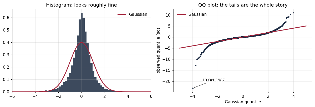
Histogram of S&P 500 daily returns against a Gaussian, and a QQ plot where the observed quantiles peel away from the Gaussian line at both ends, with Black Monday far below — S&P 500 daily returns, 1950 to 2026, in standard deviations. Left: the histogram looks roughly fine. Right: the QQ plot shows the tails, and Black Monday sits alone at the bottom.

Look at the histogram again. The centre is too tall and too narrow. That is the other half of fat tails, and it is usually forgotten: fat-tailed returns have more quiet days and more extreme days than a Gaussian with the same variance, and fewer medium ones. Most days are calmer than the model says. A few are far worse. That combination is what lulls a risk model to sleep.

How heavy: the tail index

Far enough out, the probability of a move bigger than x falls like a power of x:

P(|r| > x) ≈ C · x^−α

The exponent α is the tail index. A Gaussian falls faster than any power, so its α is effectively infinite. Smaller α, heavier tail. The consequence worth remembering: moments of order α and higher do not exist. If α is below 4, the fourth moment, which kurtosis needs, is infinite.

The Hill estimator puts a number on it: take the k largest losses and average their log distance from the next one.

α̂⁻¹ = (1/k) Σ_i=1..k [ ln X_(i) − ln X_(k+1) ]

For the S&P it comes out at about 3.0 for every reasonable choice of k. This is one of the most replicated numbers in empirical finance: Gopikrishnan, Stanley and colleagues found it across stocks and markets in 1998 and called it the inverse cubic law. For Bitcoin the estimate wobbles between about 2.4 and 4.2, which is honest: a few thousand days do not hold many tail observations.

Kurtosis is an unstable number

The S&P's excess kurtosis over the full sample is about 25. Delete one day, Black Monday, and it falls to about 11. Bitcoin's is about 16; delete the 12th of March 2020, one day out of 3,300, and it falls to about 4. A kurtosis figure is mostly a measurement of its worst day. Never compare two of them across samples and never calibrate a risk model to one.

Fact two: tails thin out as the horizon grows

Take every Binance Bitcoin price, minute by minute, from August 2017 to September 2026, almost 4.8 million minutes, and sum them into longer and longer returns. Excess kurtosis falls at every step.

Horizon	1 min	5 min	15 min	1 hour	4 hours	1 day	1 week	1 month
Excess kurtosis	120	108	72	37	21	16	2.5	2.4

The central limit theorem is at work: a daily return is the sum of 1,440 minute returns, and sums drift toward a Gaussian. Returns are not independent and their variance is barely finite, so the drift is slow. Two lessons follow. "Returns are fat-tailed" is not one statement: it depends on the clock, and a market maker holding for seconds faces a different distribution from a pension fund rebalancing monthly. And the Gaussian gets better with horizon but never good: even monthly Bitcoin returns reject normality.

Fact three: the direction of returns is barely predictable

The autocorrelation of daily returns at lags 1 to 20 is a few hundredths for both the S&P and Bitcoin. Yet the Ljung-Box test on the first ten lags rejects "no autocorrelation" for the S&P with p = 0.0006. With 19,000 observations a test can detect a correlation of 0.02. A correlation of 0.02 will not pay for your coffee.

Significant is not the same as useful

Ask the useful question instead: fit a model and see how much of tomorrow it explains, on data it has not seen.

r_t = c + φ₁ r_t−1 + … + φ_p r_t−p + ε_t

An AR(p) model, order chosen by AIC, trained on the S&P from 1950 to 1999, explains about 1% of daily variance in sample. From 2000 on, out of sample, its R² is minus 3%: its forecasts are worse than predicting the training average every day, and its direction hit rate is below the 53.7% you would get by always guessing "up". On Bitcoin it is within a tenth of a percent of zero out of sample, a hit rate of 50.5%. A coin.

Where did the in-sample 1% come from? Lag-1 autocorrelation by decade: 0.09 in the 1950s, 0.15 in the 1960s, 0.25 in the 1970s, then it fades and turns negative after 2000. The cause is plumbing. An index is built from hundreds of stocks, and in the 1960s many of them did not trade near the close, so the index used stale prices that caught up the next day. Lo and MacKinlay called it nonsynchronous trading in 1990. As markets became electronic and liquid, it disappeared. The one piece of predictability the model found was mostly a record of how old exchanges recorded prices.

Fact four: the size of returns is very predictable

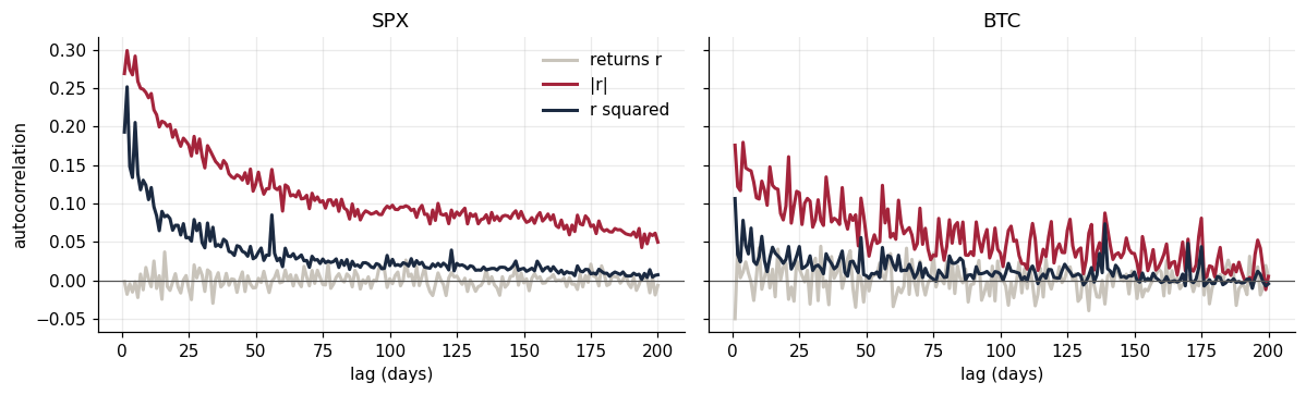
Autocorrelation out to 200 lags for S&P 500 returns, absolute returns and squared returns; returns sit at zero while absolute returns decay slowly from about 0.27 — Autocorrelation of S&P 500 daily returns (flat at zero), absolute returns and squared returns, out to 200 trading days.

This is the most important picture in the chapter. Returns: nothing. Absolute returns: 0.27 at lag 1, still 0.20 a month later and 0.09 after a hundred trading days. The direction of tomorrow is unpredictable. The size of tomorrow is very predictable. Benoit Mandelbrot described it in 1963: large changes tend to be followed by large changes, of either sign, and small changes by small changes. This is volatility clustering.

Use absolute returns when you look for it. Squaring lets a few giant days dominate the estimate, which is the kurtosis problem again.

The shuffle test

Shuffle the S&P's daily returns into random order. The shuffled series has exactly the same distribution: same mean, same volatility, same tails, same worst day. Only the order is gone.

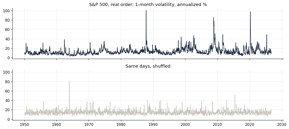
Two panels of one-month S&P 500 volatility: the real series with storms in 1987, 2008 and 2020, and the shuffled series as flat noise — One-month volatility of the S&P 500, annualized. Top: real order. Bottom: the same days, shuffled.

The worst three months in the real data lost 54% in log terms. Across 200 shuffles, the median worst quarter is minus 30%, and not one shuffle is as bad as reality. Bad days arrive together, so their losses compound instead of being diluted by calm days in between. Every risk model that treats days as independent draws from one distribution is modelling the bottom panel. The investor lives in the top one.

Modelling it: from ARCH to GARCH

Write the return as a mean plus a shock, and let the size of the shock change over time:

r_t = μ + ε_t, ε_t = σ_t z_t, z_t ~ iid, mean 0, variance 1

σ_t is today's volatility given everything known last night: the conditional volatility. Robert Engle's ARCH model (1982) says a big shock yesterday means big variance today:

σ²_t = ω + α ε²_t−1

That forgets in a day, and the memory we just measured lasts months. Tim Bollerslev (1986) added one term:

σ²_t = ω + α ε²_t−1 + β σ²_t−1

Read it as an update rule. Today's variance estimate blends a long-run level, the newest evidence (yesterday's squared shock) and the previous estimate. α is how hard new evidence moves you. β is how much of the old estimate survives.

Persistence and half-life, derived

Take expectations of the update. Since E[ε²_t−1] = E[σ²_t−1], the expected variance follows

E[σ²_t] − σ̄² = (α + β) · ( E[σ²_t−1] − σ̄² ), σ̄² = ω / (1 − α − β)

So a shock to variance decays by the factor α + β each day, the persistence, and variance reverts to the long-run level σ̄² when α + β < 1. After h days the shock is (α + β)^h of its size. Setting that to one half gives the half-life:

h_½ = ln(½) / ln(α + β)

Worked example

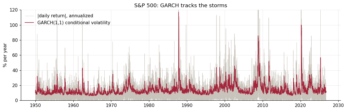
For the S&P, maximum likelihood gives α ≈ 0.09 and β ≈ 0.89, a persistence just under 0.99. The half-life comes out at about 62 trading days, roughly three months, which is exactly the slow decay in the absolute-return autocorrelation. For Bitcoin the half-life is about 26 days, at a much higher level. The volatility formula banks have used since the 1990s, the exponentially weighted RiskMetrics estimate, is this model with ω = 0 and α + β fixed at 1: no long-run level, so no mean reversion.

S&P 500 absolute daily returns with the GARCH(1,1) conditional volatility tracking the storms from 1950 to 2026 — S&P 500, 1950 to 2026: absolute daily returns (grey) and the GARCH(1,1) conditional volatility (red).

Did it work?

If the model is right, the standardized residuals ε_t/σ_t should be independent with variance one. Ljung-Box on squared residuals gives p = 0.21 for the S&P and 0.78 for Bitcoin: the clustering is captured. The S&P's excess kurtosis falls from 25 in raw returns to about 4 in the residuals. Most of its fat tail was clustering in disguise: mix calm periods and storms and the pooled distribution is fat-tailed even if each period is not.

But 4 is not zero, and Bitcoin's residual kurtosis is still about 14. The shocks themselves are fat-tailed. The fix is to draw z_t from a Student-t with ν degrees of freedom and estimate ν. The fit improves sharply again, with ν ≈ 6.4 for the S&P and ν ≈ 3.2 for Bitcoin. For a Student-t the tail index is ν, so a likelihood fit of a dynamic model and the Hill estimator on raw returns, two different methods, land in the same place.

Fact five: falls raise volatility more than rises

GARCH is symmetric: a minus 3% day and a plus 3% day raise tomorrow's variance equally. In equities that is false. The correlation between the S&P's daily return and the change in the VIX, the volatility implied by S&P options, is −0.71 over the full sample and stable across four decades. This is the leverage effect. Fischer Black's 1976 explanation: when a stock falls, the firm's debt is a bigger share of its value, so the equity is riskier. Today margin calls, forced selling and hedging demand carry most of it.

Glosten, Jagannathan and Runkle (1993) add one term that switches on only after a down day:

σ²_t = ω + ( α + γ · 1[ε_t−1 < 0] ) ε²_t−1 + β σ²_t−1

On the S&P, α falls to 0.026 and γ is 0.117. A down day moves tomorrow's variance (0.026 + 0.117) / 0.026 ≈ 5.5 times as much as an up day of the same size, after controlling for the volatility already there.

Bitcoin is a live experiment. In 2020 and 2021 its γ was negative, about −0.05: rallies raised volatility more than falls, the signature of speculative buying. From 2024 to 2026 it is about +0.08, the equity pattern. One plausible reading is that since US spot Bitcoin ETFs opened in January 2024 it is held more and more by the people who hold equities. That is a hypothesis, not a finding: the periods are short and the error bars wide. The lesson is that a stylized fact is stylized. A young market can violate one and grow into it. Measure, do not assume.

The verdict

Black Monday was a 23-sigma day using one standard deviation for 76 years, calm and storm together. Re-measure the famous crash days against a better ruler: the GJR-GARCH-t conditional volatility, estimated the evening before with only what was known then.

Day	Static sigma	Conditional sigma
S&P, 16 March 2020	13	2.4
S&P, 12 March 2020	10	2.5
S&P, 15 October 2008	9.5	2.0
S&P, 19 October 1987	23	8.6
Bitcoin, 12 March 2020	14.2	13.7

The 2008 and 2020 days arrived in the middle of storms that were already raging. Against the volatility of the moment they were ordinary bad days. The impossible numbers came from measuring a storm day with a calm-weather ruler.

Black Monday stays extreme, because early October 1987 was calm and no model built on past volatility can see a shock from calm coming. Bitcoin's March 2020 barely moves for the same reason. Under the good ruler the S&P's most extreme day is not a famous crash at all: it is the 26th of September 1955, the Monday after President Eisenhower's heart attack, minus 6.6% from a very quiet market. The deadliest days are shocks from calm, not days inside a crisis. A crisis raises the ruler. A shock from calm gives it no time to.

And how rare is a 14-sigma day under Bitcoin's fitted Student-t? About once in 66 years. Under the Gaussian, once in 10⁴¹ years.

Two mistakes, stacked

The wrong scale: a static standard deviation applied during a storm. Conditional volatility turns most famous crash days into 2 to 4 sigma events. The wrong shape: Gaussian tails, when the data says a tail index of 3 to 6. That turns the remaining extreme days from impossible into rare. Both were known long before 2007: Mandelbrot in 1963, Engle in 1982. It was not bad luck. The ruler was wrong.

What it costs: the risk number

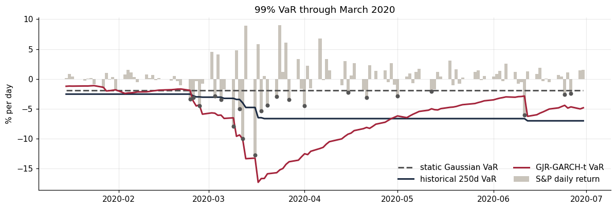
Value at Risk at 99% is the loss you expect to exceed on only 1% of days: a quantile. Expected Shortfall is the average loss on the days that do exceed it. VaR tells you where the bad tail starts. ES tells you how bad it is once you are in it.

VaR can punish diversification

Two bonds, each defaulting independently with probability 4% for a loss of 100. Hold one: the default probability is below 5%, so the 95% VaR is 0. Split the same money across both: the chance that at least one defaults is 1 − 0.96² = 7.84%, above 5%, so the VaR jumps to 50. By VaR, diversifying made you riskier.

Expected Shortfall disagrees, correctly. One bond: the worst 5% of outcomes are 4% at a loss of 100 and 1% at 0, so ES = (4 × 100 + 1 × 0) / 5 = 80. Two bonds: 0.16% lose 100 and the next 4.84% lose 50, so ES = (0.16 × 100 + 4.84 × 50) / 5 ≈ 52. A good risk measure should never say that merging two positions adds risk. Artzner and co-authors (1999) made that property, subadditivity, one of four axioms of a coherent risk measure. ES has it. VaR does not. It is part of why bank trading-book capital moved from VaR to ES.

Backtesting VaR

VaR has one great virtue: you can check it against reality. A 99% VaR should be breached on 1% of days. Four models, each using only data up to the day before, on the S&P from 1995:

99% VaR model	Days breached
Static Gaussian, calibrated once	4.30%
Rolling Gaussian, last 250 days	2.40%
Historical simulation, last 250 days	1.65%
GJR-GARCH-t, refitted yearly	1.54%

The static Gaussian is breached four times as often as it promises, and its breaches cluster: after one, the chance of another the next day is 11%. GARCH is much better and its breaches cluster far less. It is still not perfect: the Kupiec test rejects it on the S&P.

Daily S&P 500 returns through March 2020 against three 99% VaR lines: static, historical simulation and GARCH — March 2020. The static line never moves. Historical simulation reacts slowly, then stays wide for a year. GARCH widens in days and narrows as the storm fades.

What to take away

Returns have fat tails with a tail index near 3 for the S&P. Kurtosis estimates are dominated by single days.
The direction of returns is close to unpredictable. The size of returns is very predictable.
GARCH captures volatility clustering, and most of the S&P's apparent tail is clustering. The shocks that remain are still fat-tailed.
In equities, falls raise volatility more than rises. A young market can change on this.
A 25-sigma day is a scale mistake plus a shape mistake. Fix both before you trust a risk number.

Data: S&P 500 daily closes from 1950, Bitcoin daily and minute bars from Binance from August 2017, VIX daily. Every figure in this chapter was computed from that data; rerunning on refreshed data moves the second decimal.

Sources

Mandelbrot, B. (1963). The variation of certain speculative prices. Journal of Business 36(4).
Engle, R. (1982). Autoregressive conditional heteroscedasticity with estimates of the variance of United Kingdom inflation. Econometrica 50(4).
Bollerslev, T. (1986). Generalized autoregressive conditional heteroskedasticity. Journal of Econometrics 31(3).
Glosten, L., Jagannathan, R. and Runkle, D. (1993). On the relation between the expected value and the volatility of the nominal excess return on stocks. Journal of Finance 48(5).
Lo, A. and MacKinlay, C. (1990). An econometric analysis of nonsynchronous trading. Journal of Econometrics 45(1-2).
Cont, R. (2001). Empirical properties of asset returns: stylized facts and statistical issues. Quantitative Finance 1(2).
Gopikrishnan, P., Meyer, M., Amaral, L. and Stanley, H. E. (1998). Inverse cubic law for the distribution of stock price variations. European Physical Journal B 3.
Artzner, P., Delbaen, F., Eber, J.-M. and Heath, D. (1999). Coherent measures of risk. Mathematical Finance 9(3).
Tsay, R. (2010). Analysis of Financial Time Series, 3rd edition, chapters 1 and 3.

Bonton Academy is the education arm of Bonton AI, a quantitative research and development firm in Yerevan, Armenia, founded by Robert Yenokyan.