The optimizer is an error maximizer
Markowitz, eleven portfolios and eighteen years out of sample: what estimation error does to an optimizer, what shrinkage, constraints and clustering fix, and what they cannot.
By Robert Yenokyan, Bonton Academy. Published 2026-10-07. 28 minute read.
In 1952 Harry Markowitz turned "do not put all your eggs in one basket" into mathematics, and in 1990 it won him the Nobel prize. Asked late in 1997 how he invested his own retirement money, he said he had pictured his regret if stocks went way up without him, or way down with him in them, and so he split his contributions 50/50 between bonds and equities. The inventor of portfolio optimization did not use it. This chapter finds out whether he knew something the textbooks leave out.
Diversification in one line of algebra
For two assets with weights w1, w2, volatilities σ1, σ2 and correlation ρ, the portfolio variance is
Only the last term depends on ρ. At ρ = 1 the risks add and nothing cancels. Below 1 some risk cancels. Below 0 a mix can be less risky than either asset alone.
Worked example
US stocks (SPY) and ten-year Treasuries (IEF), 2007 to 2026: volatilities 19.6% and 6.9% a year, correlation of daily returns −0.29. The 50/50 mix has 9.4% volatility against an average of 13.3%: diversification removed almost a third of the risk for free. The lowest-risk mix, 17% stocks and 83% bonds, has 5.8%, less than holding bonds alone.
The universe for the rest of the chapter is 17 ETFs: US, European and emerging-market equity, four US sectors, real estate, Treasuries at two maturities, inflation-linked bonds, corporate and high-yield credit, gold and commodities. The data starts on the 11th of April 2007, so 2008 is inside it. Short-term Treasuries are in the data and out of every portfolio: their raw Sharpe ratio of 1.19 falls to 0.21 against T-bills. It is cash in a costume. All Sharpe ratios below are measured on returns over T-bills.
One number to remember. With 19 years of data, how many of the 17 funds have an average excess return you can tell apart from zero at a t-statistic of 2? Four. Technology, health care, gold and the S&P 500. For the other thirteen, two decades of data cannot tell you whether the expected return is positive.
The frontier, written as a convex program
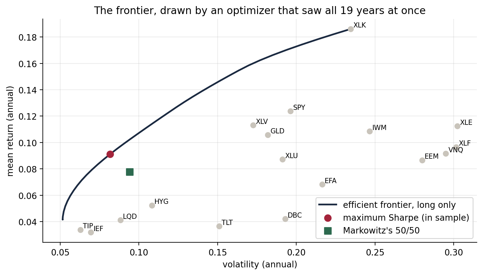
The maximum Sharpe portfolio on this frontier scores 0.93 and puts nearly everything in four funds: 46% ten-year Treasuries, 25% technology, 18% gold, 10% health care. It chose technology because technology did well in exactly the years it is judged on. Everything after this is about how much of that survives when the optimizer only sees the past.
In practice you write the problem as
subject to Σi wi = 1, 0 ≤ w ≤ u, Aw ≤ b
Expected return, minus a risk penalty, minus a trading penalty, with a budget, no shorting, a cap per position and group limits such as "equity at most 60%". A quadratic objective with linear constraints is convex, and convex problems have a property worth more than speed: every local optimum is the global one, and the solver can prove it. The L1 trading penalty is the lasso penalty, and it works for the same reason: it pushes most changes to exactly zero, so the portfolio trades rarely and in few names.
Infeasible is an answer
Three client profiles under one policy (at most 25% in one fund, 60% equity, 15% real assets, 30% credit) at 6%, 9% and 12% target volatility are three calls of the same solver. Ask for 5% and the solver says infeasible: under that policy nothing goes below about 5.6%. When a client asks for "no more than 5% risk and at least 40% equity", this is how you find out it cannot be done.
Every constraint can only lower the in-sample answer: unconstrained, the optimizer holds three funds with the largest at 61% and a Sharpe of 0.857; with the 25% cap, five funds and 0.854; with group limits, 0.853. Here they cost almost nothing. What they do out of sample is a different question.
How well do we know the inputs?
The optimizer treats μ and Σ as known. They are estimates, and not equally good ones.
The precision of a mean depends on how many years you have. The precision of a volatility depends on how many observations you have. Sample every minute instead of every day and you get far more observations and zero more years.
Worked example
A market with a 6% excess return and 18% volatility. The t-statistic of its mean after T years is t = μ√T / σ. Setting t = 2 gives T = (2σ / μ)2 = (2 × 18 / 6)2 = 36 years. On our data: technology needs 7.5 years, the S&P 13, emerging markets 61, long Treasuries 195 and commodities 202. Meanwhile one year of daily data pins any fund's volatility to within about 4.5%, relative.
The mean-variance formula is most sensitive to μ, which is the input we know least.
The error maximizer
Richard Michaud put the problem in one line in 1989: the optimizer cannot tell a high return that is real from a high return that is estimation error, so it overweights both, and the asset with the biggest lucky error gets the biggest weight. He called mean-variance optimizers "estimation-error maximizers". Two tests.
Test 1: the same year, two hundred times
Take the most recent year of returns and build 200 alternative versions with a block bootstrap: cut it into 20-day blocks, draw blocks at random, glue them back. Every version is a year that could have happened in the same market. Solve for the maximum Sharpe portfolio on each.
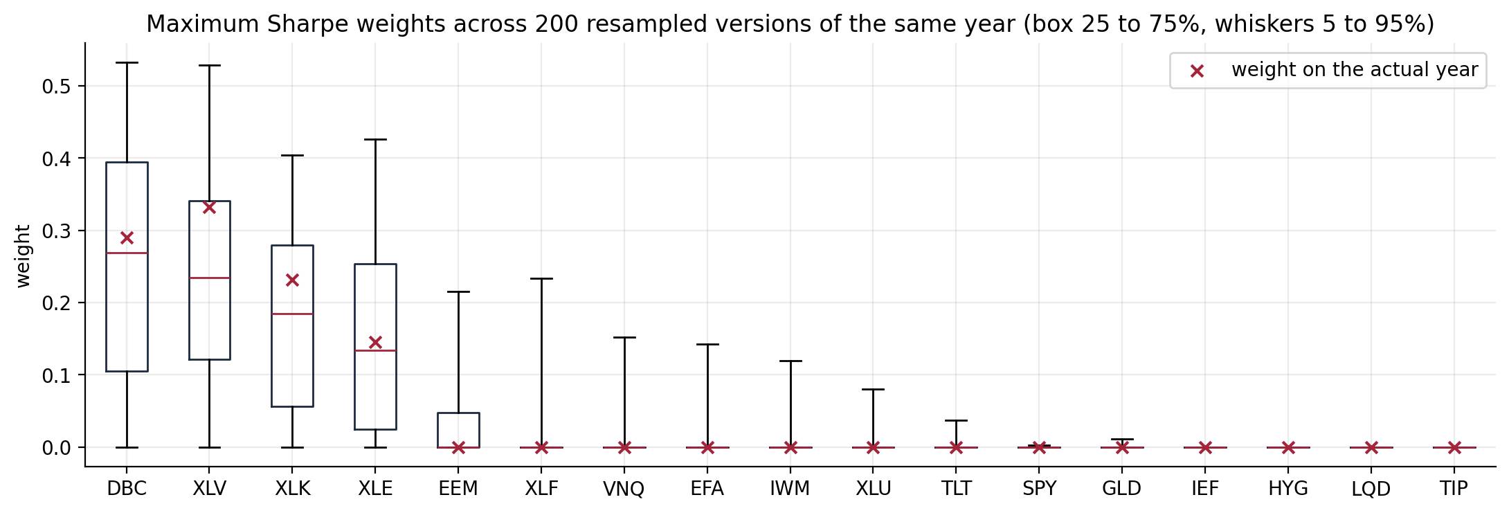
On the real year the largest holding is health care at 33%. Across the resampled years the largest holding was nine different funds: commodities in 38% of them, health care in 34%, energy 12%, technology 8%. Same market, statistically indistinguishable histories, and the optimizer cannot decide what it mostly wants to own. The width of those boxes is not information about the market. It is noise, amplified.
Test 2: promised against delivered
Take μ away completely. The minimum variance portfolio uses only Σ, the input we estimate well, and without the long-only constraint it has a closed form:
Use 48 large US stocks. Every month from 2012 to 2026, estimate Σ from the last 60 trading days, solve and record the volatility the portfolio promises on the data it was fitted to and the volatility it delivers the next month. A 48 × 48 covariance matrix has 48 × 49 / 2 = 1,176 distinct numbers. We are estimating them from 60 days.
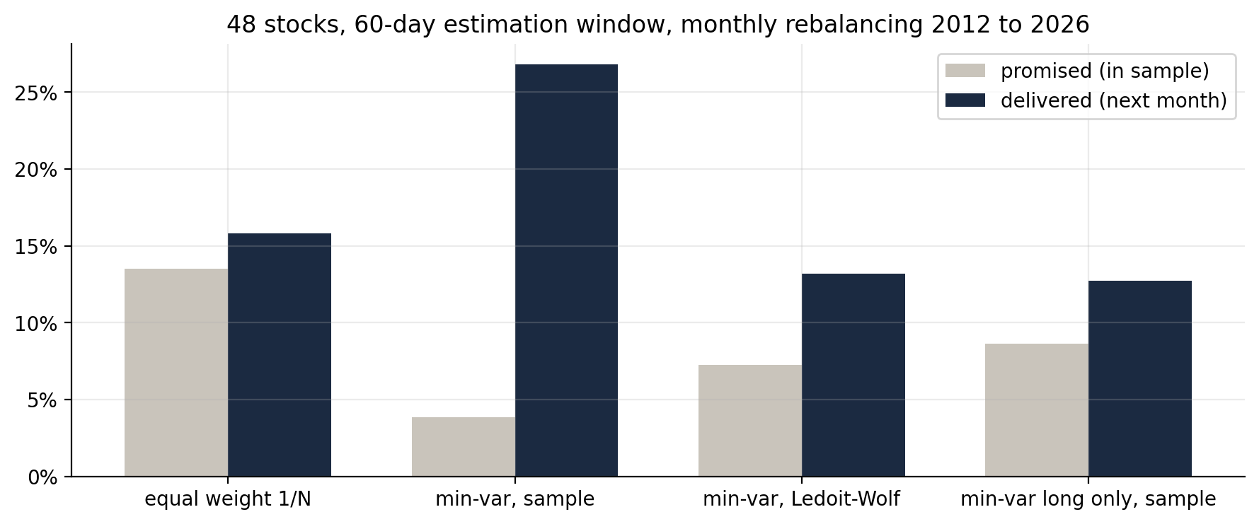
It promises 3.9% volatility for a portfolio of stocks, lower than a bond fund. It delivers 26.8%, seven times the promise, by holding 8.8 times its capital in long and short positions. Buying all 48 equally promised 13.5% and delivered 15.8%. With 60 days of data the sample covariance contains directions where risk looks almost zero. They are mostly noise. The optimizer found them and bet the house on them.
Anyone who has trained a model will recognise the picture: training error tiny, test error enormous, too many parameters for the data. It is overfitting, and the standard cures for overfitting apply.
Fix 1: regularize
Ledoit and Wolf (2004) did for a covariance matrix what a ridge penalty does for a regression: accept a little bias to cut a lot of variance. Pull the sample covariance S toward a boring target, and let a closed-form formula choose how far:
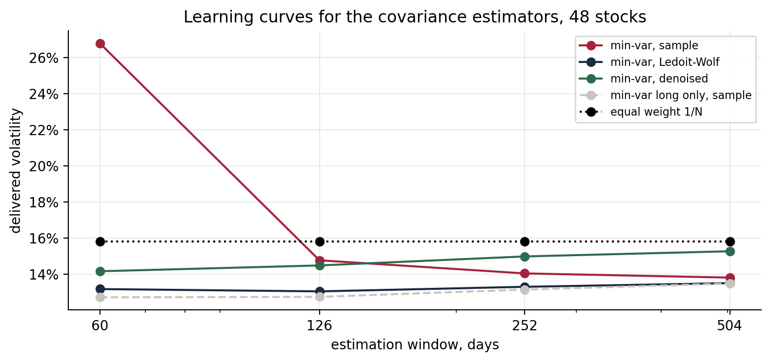
At 60 days the raw estimator delivers 26.8% and Ledoit-Wolf 13.2%: shrinkage halved the realized risk. As the window grows the gap closes and the shrinkage intensity the formula picks falls from 0.18 at 60 days to 0.03 at two years. More data earns the sample more trust, exactly as a well-tuned ridge penalty does.
The dashed line is long-only minimum variance with no shrinkage at all, and it is the best line on the chart: 12.7% at 60 days. Jagannathan and Ma proved why in 2003. Forbidding short positions is equivalent to solving the unconstrained problem with a covariance matrix in which the estimates that would have produced short positions are shrunk. The constraint is a regularizer. Constraints cost you in sample. Out of sample they are regularization.
Fix 2: throw away the noise
Random matrix theory says what the eigenvalues of a correlation matrix look like when the data is pure noise. For N assets and T observations, Marchenko and Pastur (1967) showed they fall inside
For 48 stocks and 252 days, q = 0.19 and the noise edge is λ+ ≈ 2.06. Shuffle each stock's returns in time independently, which keeps every distribution and destroys every relationship, and the largest eigenvalue is 1.84, inside the band as the theory says. On the real data four eigenvalues stand out: 8.7, 6.7, 5.3 and 3.5. The other 44 sit at or below the edge, the same picture Laloux, Cizeau, Bouchaud and Potters found for the S&P 500 in 1999.
Principal components show what the four are. The first loads every stock with the same sign, +0.10 to +0.18: the market, explaining 37% of all daily movement. The second puts five oil and gas producers at one end and five power utilities at the other, without ever being told the sectors. On the 9th of March 2020, the day oil collapsed, our energy stocks lost 26% on average and utilities 5.6%.
So keep the real directions, flatten the rest to their average and re-optimize. It beats the raw estimator at 60 days, 14.2% against 26.8%. It never beats Ledoit-Wolf, and at one and two years it is worse than the raw sample. A likely reason is that clipping at the textbook edge also flattens weaker sector directions that are real. An elegant method is not evidence that it works on your data. Test it before you believe it.
Fix 3: let the data find the structure
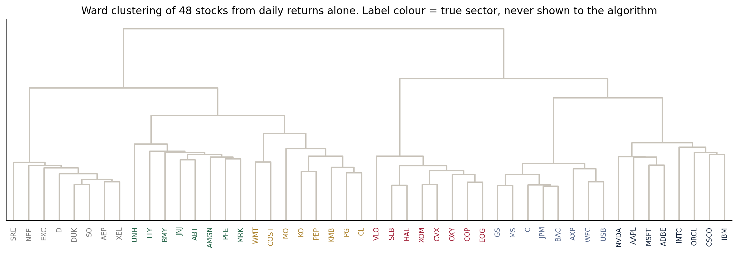
Shrinkage and denoising still invert a covariance matrix, and inversion is where errors get amplified. Clustering never inverts anything. Using only daily returns, with distance built from correlation, Ward linkage puts every one of the 48 stocks in its correct sector: an adjusted Rand index of 1.0. The linkage rule matters: complete linkage scores 0.60, average 0.52 and single linkage 0.29, because single linkage merges two groups when their closest pair is close and builds long chains. Hierarchical Risk Parity, as López de Prado published it in 2016, uses single linkage.
HRP in three steps: cluster and order the assets so similar ones sit together; split the list in half and give each half money in inverse proportion to its risk; repeat inside each half. Weights are always positive and never extreme. No matrix is inverted. On our 17 funds it puts about three quarters into the four lowest-risk bond and credit funds.
The race
Eleven portfolios, 17 funds, rules fixed before the run. At each month end every portfolio estimates what it needs from the previous 252 trading days only, then holds for a month. The race runs from May 2008 to September 2026, eighteen years out of sample through 2008, 2020 and 2022, with 10 basis points of cost on every unit traded. One change was made after a trial run, and it is disclosed: short-term Treasuries came out and Sharpe moved to excess returns. Nothing was tuned on results.
| Portfolio | Uses | Sharpe |
|---|---|---|
| Markowitz's 50/50 (SPY, IEF) | nothing | 0.67 |
| Maximum Sharpe, 20% cap | μ, Σ | 0.61 |
| Mean-variance, caps and turnover penalty | μ, Σ | 0.59 |
| Maximum Sharpe, textbook | μ, Σ | 0.58 |
| Risk parity | Σ | 0.55 |
| Inverse volatility | σ | 0.52 |
| Equal weight, 1/N | nothing | 0.50 |
| Hierarchical risk parity | Σ | 0.38 |
| Minimum variance, three estimators | Σ | 0.32, 0.21, 0.20 |
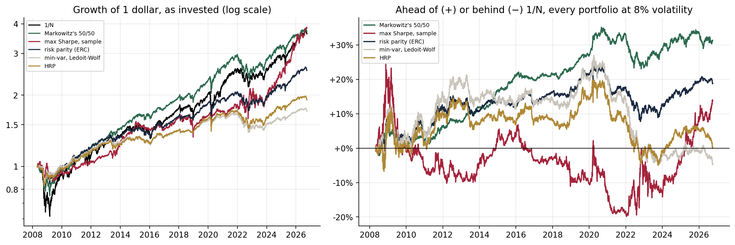
Four readings of that table.
Turnover. The portfolios that use the mean trade four to six times their whole value every year; the textbook one 5.8 times, 1/N 0.3. Its largest holding changed in 60 of 221 months. That is the error maximizer filmed over eighteen years.
Why the mean users ranked well. A one-year trailing mean is a momentum signal. Going into 2022 the textbook portfolio held on average 42% energy and 20% commodities after a strong 2021, and in 2022 energy rose another 64% while nearly everything else fell. Momentum across asset classes is documented (Moskowitz, Ooi and Pedersen, 2012). It is also exactly the kind of story that is easy to find after the fact. And minimum variance did what it promises, the lowest volatility in the table at 5.2%, by holding about 87% in bond funds. It is a risk objective. Judging it on Sharpe is judging a fish on climbing.
Constraints. Out of sample the capped maximum Sharpe beat the uncapped one, 0.61 against 0.58, with turnover of 4.1 instead of 5.8 and an average largest position of 20% instead of 57%. The constraint that cost almost nothing in sample paid out of sample.
Is any of it real? A Sharpe ratio is a mean divided by something, and means need decades. Bootstrap each portfolio's Sharpe difference against 1/N, keeping the two return series paired:
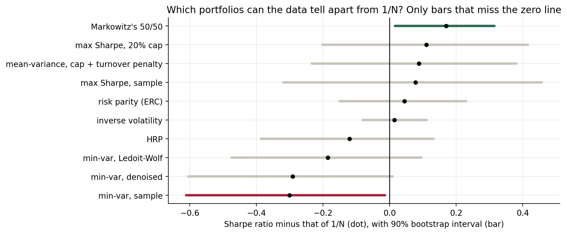
Every grey bar crosses zero, including every portfolio that used the mean. The textbook maximum Sharpe beat 1/N by 0.08 with an interval from −0.32 to +0.46. Only two bars miss zero: the 50/50, better, with an interval of 0.02 to 0.31, and raw minimum variance, worse. Ten tests at 90% should produce about one such result by chance, and the 50/50 only just clears. DeMiguel, Garlappi and Uppal reached the same conclusion in 2009 with 14 optimizers on seven datasets, and estimated that mean-variance on 25 assets would need more than 3,000 months of data to reliably beat 1/N. Two hundred and fifty years.
2022: the year the hedge stopped hedging
Every portfolio holding bonds leaned on one number: the negative correlation between stocks and bonds. One-year rolling, it went as low as −0.73. At the end of 2021 it was −0.09 and at the end of 2022 +0.19. Inflation was high and rates rose fast, which pushes bond prices and stock prices down together: SPY lost 18.2%, IEF 15.2% and long Treasuries 31.2%. Every covariance matrix built on the years before had learned a negative sign. A correlation is an estimate from a period, not a law.
Audit the winner with your own test
The 50/50 tops the table. But why SPY and IEF? Because, writing in 2026, we know American large caps were among the best equity holdings of these years and Treasuries their best partner. That is hindsight. So pair every equity fund with every bond and credit fund: 45 possible 50/50 portfolios, same race, same costs.
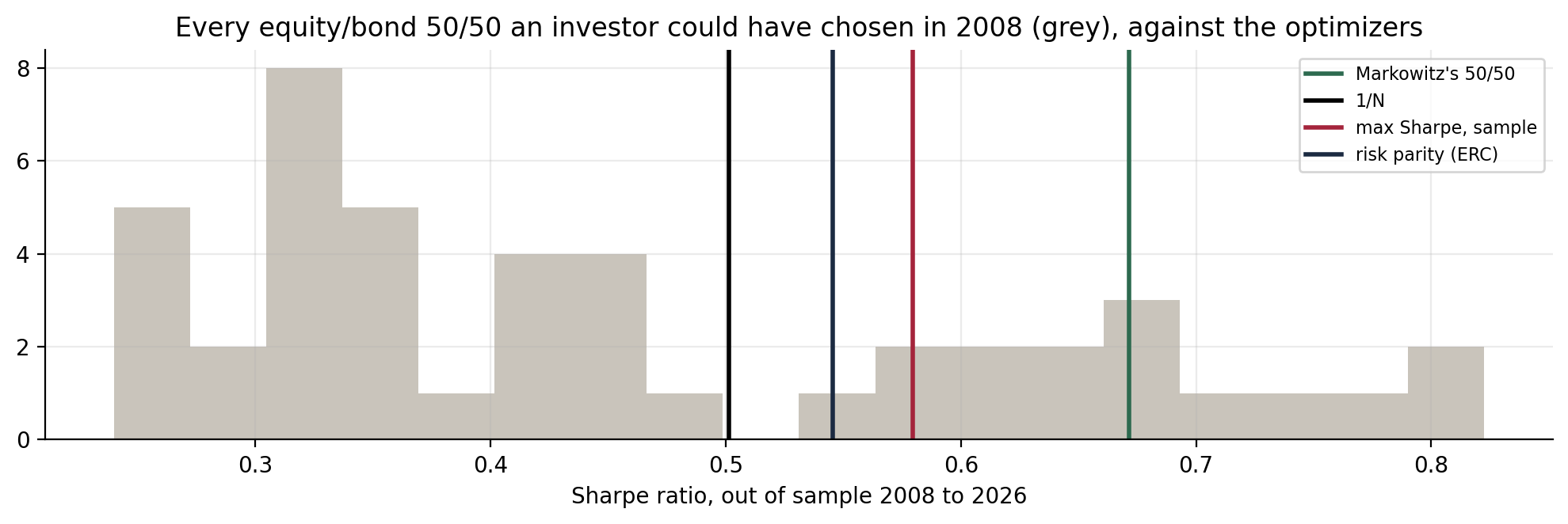
The median 50/50 scores 0.43. The best, technology with Treasuries, 0.82. The worst, emerging markets with inflation-linked bonds, 0.24. SPY and IEF rank seventh of 45, and equal weighting beats 67% of them.
The verdict
The optimizer is an error maximizer: it promised 4% volatility and delivered 27%, and changed its mind with every resample of the same year. Machine learning helps where the problem is estimation, and only there: shrinkage and constraints closed the gap between promised and delivered risk, and clustering found real structure without inverting anything. None of it turned one year of past means into a reliable forecast. On eighteen years of data, nothing built from estimates could be shown to beat a rule that uses none. Markowitz never claimed his 50/50 was optimal. He chose a rule that needs no estimates, and the data has no answer that beats it with confidence.
That does not make optimization useless. Given only the covariance and asked to cut risk on the 48 stocks, long-only and shrunk, it cuts volatility from 15.7% to 12.9%, and the whole bootstrap interval says 15% to 21% less risk; in March 2020 it lost 8.3% where equal weight lost 14.2%. Optimization is not a source of returns. It is an amplifier. Good input, good portfolio. One year of past means, amplified noise.
What to take away
- The mean is the input you know least, and the optimizer leans on it hardest.
- An unregularized optimizer overfits like any model. Constraints and shrinkage are regularization.
- Test the elegant method before you believe it. Denoising looked beautiful and lost here.
- Audit your own winner with the test you used on everyone else.
Data: daily adjusted closes for 18 US-listed ETFs from April 2007 to October 2026, and a 48-stock panel from 2012 used for risk and clustering only (it is survivor-biased, so no return claims are drawn from it). Bootstrap figures depend on the random seed at the second decimal.
Sources
- Markowitz, H. (1952). Portfolio selection. Journal of Finance 7(1).
- Michaud, R. (1989). The Markowitz optimization enigma: is 'optimized' optimal? Financial Analysts Journal 45(1).
- Jagannathan, R. and Ma, T. (2003). Risk reduction in large portfolios: why imposing the wrong constraints helps. Journal of Finance 58(4).
- Ledoit, O. and Wolf, M. (2004). A well-conditioned estimator for large-dimensional covariance matrices. Journal of Multivariate Analysis 88(2).
- Marchenko, V. and Pastur, L. (1967). Distribution of eigenvalues for some sets of random matrices. Mathematics of the USSR-Sbornik 1(4).
- Laloux, L., Cizeau, P., Bouchaud, J.-P. and Potters, M. (1999). Noise dressing of financial correlation matrices. Physical Review Letters 83.
- López de Prado, M. (2016). Building diversified portfolios that outperform out of sample. Journal of Portfolio Management 42(4).
- DeMiguel, V., Garlappi, L. and Uppal, R. (2009). Optimal versus naive diversification: how inefficient is the 1/N portfolio strategy? Review of Financial Studies 22(5).
- Moskowitz, T., Ooi, Y. H. and Pedersen, L. H. (2012). Time series momentum. Journal of Financial Economics 104(2).